7 ways to label a cluster plot in Python

This tutorial shows you 7 different ways to label a scatter plot with different groups (or clusters) of data points. I made the plots using the Python packages matplotlib and seaborn, but you could reproduce them in any software. These labeling methods are useful to represent the results of clustering algorithms, such as k-means clustering, or when your data is divided up into groups that tend to cluster together.

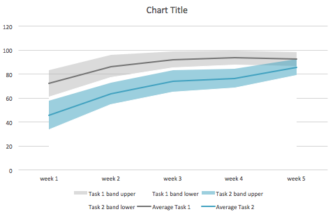
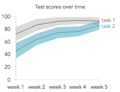
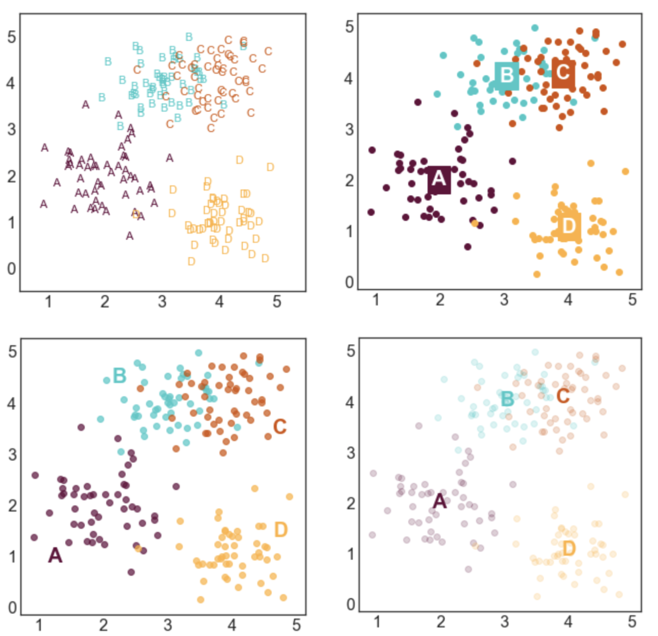
Here's a sneak peek of some of the plots:

You can access the Juypter notebook I used to create the plots here. I also embedded the code below.

First, we need to import a few libraries and define some basic formatting:

import pandas as pd
import numpy as np

import seaborn as sns
import matplotlib.pyplot as plt
%matplotlib inline

#set font size of labels on matplotlib plots
plt.rc('font', size=16)

#set style of plots
sns.set_style('white')

#define a custom palette
customPalette = ['#630C3A', '#39C8C6', '#D3500C', '#FFB139']
sns.set_palette(customPalette)
sns.palplot(customPalette)

CREATE LABELED GROUPS OF DATA

Next, we need to generate some data to plot. I defined four groups (A, B, C, and D) and specified their center points. For each label, I sampled nx2 data points from a gaussian distribution centered at the mean of the group and with a standard deviation of 0.5.

To make these plots, each datapoint needs to be assigned a label. If your data isn't labeled, you can use a clustering algorithm to create artificial groups.

#number of points per group
n = 50

#define group labels and their centers
groups = {'A': (2,2),
          'B': (3,4),
          'C': (4,4),
          'D': (4,1)}

#create labeled x and y data
data = pd.DataFrame(index=range(n*len(groups)), columns=['x','y','label'])
for i, group in enumerate(groups.keys()):
    #randomly select n datapoints from a gaussian distrbution
    data.loc[i*n:((i+1)*n)-1,['x','y']] = np.random.normal(groups[group], 
                                                           [0.5,0.5], 
                                                           [n,2])
    #add group labels
    data.loc[i*n:((i+1)*n)-1,['label']] = group

data.head()

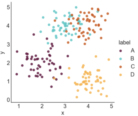
STYLE 1: STANDARD LEGEND

Seaborn makes it incredibly easy to generate a nice looking labeled scatter plot. This style works well if your data points are labeled, but don't really form clusters, or if your labels are long.

#plot data with seaborn
facet = sns.lmplot(data=data, x='x', y='y', hue='label', 
                   fit_reg=False, legend=True, legend_out=True)

STYLE 2: COLOR-CODED LEGEND

This is a slightly fancier version of style 1 where the text labels in the legend are also color-coded. I like using this option when I have longer labels. When I'm going for a minimal look, I'll drop the colored bullet points in the legend and only keep the colored text.

#plot data with seaborn (don't add a legend yet)
facet = sns.lmplot(data=data, x='x', y='y', hue='label', 
                   fit_reg=False, legend=False)

#add a legend
leg = facet.ax.legend(bbox_to_anchor=[1, 0.75],
                         title="label", fancybox=True)
#change colors of labels
for i, text in enumerate(leg.get_texts()):
    plt.setp(text, color = customPalette[i])
    

STYLE 3: COLOR-CODED TITLE

This option can work really well in some contexts, but poorly in others. It probably isn't a good option if you have a lot of group labels or the group labels are very long. However, if you have only 2 or 3 labels, it can make for a clean and stylish option. I would use this type of labeling in a presentation or in a blog post, but I probably wouldn't use in more formal contexts like an academic paper. 

#plot data with seaborn
facet = sns.lmplot(data=data, x='x', y='y', hue='label', 
                   fit_reg=False, legend=False)

#define padding -- higher numbers will move title rightward
pad = 4.5

#define separation between cluster labels
sep = 0.3

#define y position of title
y = 5.6

#add beginning of title in black
facet.ax.text(pad, y, 'Distributions of points in clusters:', 
              ha='right', va='bottom', color='black')

#add color-coded cluster labels
for i, label in enumerate(groups.keys()):
    text = facet.ax.text(pad+((i+1)*sep), y, label, 
                         ha='right', va='bottom',
                         color=customPalette[i])

STYLE 4: LABELS NEXT TO CLUSTERS

This is my favorite style and the labeling scheme I use most often. I generally like to place labels next to the data instead of in a legend. The only draw back of this labeling scheme is that you need to hard code where you want the labels to be positioned. 

#define labels and where they should go
labels = {'A': (1.25,1),
          'B': (2.25,4.5),
          'C': (4.75,3.5),
          'D': (4.75,1.5)}

#create a new figure
plt.figure(figsize=(5,5))

#loop through labels and plot each cluster
for i, label in enumerate(groups.keys()):

    #add data points 
    plt.scatter(x=data.loc[data['label']==label, 'x'], 
                y=data.loc[data['label']==label,'y'], 
                color=customPalette[i], 
                alpha=0.7)
    
    #add label
    plt.annotate(label, 
                 labels[label],
                 horizontalalignment='center',
                 verticalalignment='center',
                 size=20, weight='bold',
                 color=customPalette[i]) 

STYLE 5: LABELS CENTERED ON CLUSTER MEANS

This style is advantageous if you care more about where the cluster means are than the locations of the individual points. I made the points more transparent to improve the visibility of the labels.

#create a new figure
plt.figure(figsize=(5,5))

#loop through labels and plot each cluster
for i, label in enumerate(groups.keys()):

    #add data points 
    plt.scatter(x=data.loc[data['label']==label, 'x'], 
                y=data.loc[data['label']==label,'y'], 
                color=customPalette[i], 
                alpha=0.20)
    
    #add label
    plt.annotate(label, 
                 data.loc[data['label']==label,['x','y']].mean(),
                 horizontalalignment='center',
                 verticalalignment='center',
                 size=20, weight='bold',
                 color=customPalette[i]) 

STYLE 6: LABELS CENTERED ON CLUSTER MEANS (2)

This style is similar to style 5, but relies on a different way to improve label visibility. Here, the background of the labels are color-coded and the text is white.

#create a new figure
plt.figure(figsize=(5,5))

#loop through labels and plot each cluster
for i, label in enumerate(groups.keys()):

    #add data points 
    plt.scatter(x=data.loc[data['label']==label, 'x'], 
                y=data.loc[data['label']==label,'y'], 
                color=customPalette[i], 
                alpha=1)
    
    #add label
    plt.annotate(label, 
                 data.loc[data['label']==label,['x','y']].mean(),
                 horizontalalignment='center',
                 verticalalignment='center',
                 size=20, weight='bold',
                 color='white',
                 backgroundcolor=customPalette[i]) 

STYLE 7: TEXT MARKERS

This style is a little bit odd, but it can be effective in some situations. This type of labeling scheme may be useful when there are few data points and the labels are very short.

#create a new figure and set the x and y limits
fig, axes = plt.subplots(figsize=(5,5))
axes.set_xlim(0.5,5.5)
axes.set_ylim(-0.5,5.5)

#loop through labels and plot each cluster
for i, label in enumerate(groups.keys()):

    #loop through data points and plot each point 
    for l, row in data.loc[data['label']==label,:].iterrows():
    
        #add the data point as text
        plt.annotate(row['label'], 
                     (row['x'], row['y']),
                     horizontalalignment='center',
                     verticalalignment='center',
                     size=11,
                     color=customPalette[i]) 

How to assign different colors to different conditions in Excel graphs

This post was originally published on May 12, 2014.

Excel is a great program to use if you don’t require complicated graphs and if you use their default formatting (which you shouldn’t!). However, if you need more advanced formatting, making graphs in Excel can become complicated. It’s not impossible though — there are ways to manipulate Excel to create beautiful, custom charts. 

In this tutorial, I describe how to conditionally format graphs in Excel. Conditional formatting is useful when you have two or more conditions that you want to format differently. For example, if you have data from a patient group and a control group and you want to display their data in different colors, sizes, or shapes. Excel does let you format data points individually, but applying the same format to every data point in each condition can quickly become labor intensive. Here's an example where two groups of participants are labeled with different colors:

STEP 1: ORGANIZE YOUR DATA

To begin, organize all your data in columns. The first column should contain dummy codes for your different conditions. For example, if you have three conditions, you’ll use the numbers 1,2, and 3 to represent your conditions. The remaining columns should contain your variables that you plan to plot — you should have two columns if you want to make a scatter chart and one column if you are making a bar chart or something similar. In this example, I have two groups: a control group, which I dummy coded with 1, and a patient group, which I dummy coded with 2. Each subject has a response time that is listed in column B:

STEP 2: SEPARATE DATA ACCORDING TO CONDITION TYPE

This step includes the meat of the tutorial. First, create new columns for each condition type and each variable (if you have 2 conditions and 1 variable, you’ll need 2 new columns and if you have 3 conditions and 2 variables, you’ll need 6 new columns). In each column, type an IF statement with the following parameters:

=IF(condition = dummy code, variable, NA() )

where "condition" is the cell containing your dummy code, "dummy code" is the actual number of your dummy coding (this number will change in each column), and "variable" is the cell containing your data. So in our example, we’ll use the following IF statements:

In the first new column:    =IF(A6=1,B6,NA())

In the second new column:    =IF(A6=2,B6,NA())

Finally, apply the formatting to all your data by highlighting the cells containing your IF statements and dragging the blue box in the lower righthand corner all the way down to the end of your data.

STEP 3: CREATE A GRAPH

At this point, you can create whatever type of graph you need — this conditional formatting technique can be used to create a wide variety of graphs. In this example, I created a simple bar chart to visualize subjects’ response times according to condition type.

To create a bar chart, click on the charts tab in the Excel ribbon. Highlight the data in the new columns you just created (the columns with the #N/A values), click on the Bar icon, and select clustered bar chart. Now when you click on a datapoint in the graph, it will highlight all of the other datapoints that belong to the same condition. You can format the datapoints in each condition separately. 

To make the spacing of the bars uniform, right click on the data series and select format data series. Change the overlap to 100% and the gap width to 100%. To finish formatting, I removed the gridlines, added a title and and x axis label, changed the typeface of the axes and labels to Avenir, changed the color of the bars to a neutral gray for the controls and a teal for the patients, and removed all shadows and other special effects. I also removed the y-axis labels since the subject number does not matter in this case. Here’s the finished graph:

You can use the same conditional formatting technique to create scatter plots too. Here's an example of how to set up the data:

And here's what the formatted scatter plot looks like:

How to make shaded error bands in Excel

This tutorial describes how to create error bands or confidence intervals in line graphs using Excel for Mac. Excel has a built-in capability to add error bars to individual time points in a time series, but doing so can make the graph look messy and can conceal the overall shape or trend of the time series’ error. Shaded error bands provide good estimates of uncertainty without distracting from the time series. Creating error bands in Excel isn’t as straight forward as creating individual error bars — but never fear, this tutorial will show you how.

Here’s an sneak-peek of a two time series and their associated shaded error bands:

STEP 1: FORMAT YOUR DATA

First, you’ll need to organize your data according to the following format:

The rows should contain the averages and uncertainty measurements associated with each condition and the columns should contain measurements over time. In the example above, I use standard error but you could also use a confidence interval, standard deviation, variance, or any other measurement of uncertainty.

Below the rows containing the averages and standard deviations, we will add additional rows for the upper and lower bound of each error band.

STEP 2: FIND THE UPPER AND LOWER BOUNDS OF EACH ERROR BAND

To find the upper bound of an error band, simply add the error to the average. So in our example, I added the average (cell C2) and the standard error (cell c4).

Similarly, subtract the error from the average to find the lower bound. In this example, I subtracted the standard error (cell c4) from the average (cell C2).

Find the upper and lower error bound for every time series in your data. Finally, apply the formatting to the other columns by highlighting the cells containing the upper and lower error bounds, and dragging the blue square on the bottom right of the box across the rest of your data columns.

STEP 3: GRAPH THE TIME SERIES

Select the time series averages and then click the option key and select the error band data too:

 Create a line graph by clicking on the Charts tab in the Excel ribbon, clicking the Line icon under the Insert Chart area, and selecting the Marked Line plot. Switch the rows & columns of the chart by clicking the column button (the icon with the table and highlighted column)  in the data section of the Charts ribbon. Next, remove the time series associated with the standard error by clicking on the lines and pressing delete. Your graph should look similar to this:

STEP 4: ADD THE ERROR BANDS

Right click on one of the lines associated with an upper or lower error band bound and select Change series chart type. Click the Area icon under the Change Chart Type section and select the Area plot. Repeat this step for every upper and lower bound. Now your graph should look like this:

For every lower bound:

•  change the fill to white
• change the line color to white
• remove the shadow

For every upper bound:

•  change the line color to “no fill”
• remove the shadow 
• set the transparency to 50% (shape fill -> more fill colors... -> move the opacity slider to 50%)
• change the fill color to a lighter version of your time series color

Now your graph should look like this:

STEP 5: FORMAT THE GRAPH

Finally, remove the legend labels associated with the error bounds by selecting each label and pressing delete. Remove the grid lines by selecting a grid line and pressing delete. Format the graph to your liking. Here is an example of a fully formatted graph: 

How to 3D-print your brain

This post was originally published on May 11, 2015. The tutorial was updated on November 20, 2017.

A few weeks ago, I made a 3D model of my brain and sent it to Shapeways to get it 3D-printed. My little brain arrived a few days ago and I’m blown away by how good it turned out. I don’t want to be overly dramatic, but I think this is one of the coolest things I’ve ever done. The whole process was relatively straight forward once I figured out the best program to use. I wrote a step-by-step tutorial of what I did below in case you want to print your brain too.

And if you want a brain on your desk and you don’t care whose it is, you can order a 3D model of my brain here.

INSPIRATION & Background

I have a deep fascination of the human brain and I’ve wanted a 3D model of my brain for quite some time. I considered using a modeling software (like Blender) to create my own 3D brain model based on my MRI scans, but I quickly abandoned that idea when I imagined manually outlining the cortex one slice at a time.

A few months ago, one of my friends posted a link to a company that sells custom brain models that range from $165.00 (for half scale models) to $342.00 (for full scale models). I was tempted to order a model, but I finally decided that it was too expensive. I love brains, but not quite that much.

Then, a few weeks ago, I came across this blog post that included do-it-yourself instructions for creating a 3D model of your brain for 3D printing. The neuroscientist and cheapskate in me rejoiced. My computer was being serviced so I bookmarked the page and waited until I got my laptop back.

When I finally sat down to follow the tutorial, I found that it left out some crucial steps and required a lot of manual editing. I spent a few hours looking at other tutorials, downloading software packages, and trying to create a halfway decent 3D model, but none of the models I created had anywhere near the level of detail I wanted.

Finally, I found this tutorial which describes how to create a 3D model using Freesurfer. I had been wanting to learn how to use Freesurfer for awhile, so it was a win/win. The tutorial is pretty thorough, but it didn’t explain the installation of Freesurfer, which ended up being somewhat complicated. In case you’re like me and haven’t used Freesurfer before, I added detailed information about how to download and install Freesurfer below. If you already use Freesurfer, you are in luck! You are only a few steps away to creating your own 3D brain model (you can skip to the “Create the 3D brain model” section).

STEP 1: GET YOUR BRAIN SCANNED

• First, you need to get a T1 anatomical scan of your brain with MRI. Okay, I understand that that’s easier said than done, but there’s no way around it.
• Add all of your DICOM files from the T1 anatomical scan into one folder. My folder is named “t1_mprage_DICOM.”

STEP 2: DOWNLOAD AND INSTALL FREESURFER

If you already have Freesurfer installed, skip to the next section. 

• Download Freesurfer here. I downloaded the freesurfer-Darwin-lion-stable-pub-v5.3.0.dmg  file.
• If you don’t already have XQuartz installed, you’ll have to download and install it in order to use Freesurfer. Download the latest release here.
• Install Freesurfer by following the detailed instructions here. You should come to a screen that looks like this:

• In order to get everything set up correctly, you have to modify your .profile file (the first time I tried to install Freesurfer I didn’t read this this page (oops), and I ran into trouble later on). Your computer may be set up differently, so these steps may not apply to you.
• Modify your .profile file by typing the following command in the terminal window (I already have a .profile file that is named .bash_profile so I opened that file):

        >> touch ~/.bash_profile; open ~/.bash_profile 

• Copy the set of command lines from the install window and paste it at the bottom of the file that pops up. My file looks like this:

• Get an installation key by filling out the form here. You will receive an email containing information about your license. Copy the text in between the –CUT HERE– lines and paste them into a new TextEdit file. Convert the file into a plain text file by clicking Format –> Make plain text. Name the file ‘license.txt’ and save it in the Freesurfer folder.

STEP 3: CREATE THE 3D BRAIN MODEL

• In your terminal window, type the following command to set up Freesurfer:

    >> source /Applications/freesurfer/SetUpFreeSurfer.sh

• We will use the function called recon-all to create the 3D brain model. Detailed information about the recon function is available here.
  The function uses the following format:

    >> recon -all -i <DICOM file> -subjid <folder name> -all

Replace the <DICOM file> part with the path to any one of your DICOM files (and not the folder that holds all the files). Replace <folder name> with the name you want to call the folder that will contain all of the output files. The folder will be added to the same directory that your DICOM folder is in. My function looked like this:

    >> recon-all -i Documents/my_brain/t1_mprage_DICOM/IM-0001-0001.dcm -subjid me_in_3D –all

• Enter the command into terminal and press enter to start the analysis. The analysis takes a long time. The reconstruction took 8 hours on my computer, but others estimate that it can take between 10 and 20 hours. Make sure that you turn off your computer’s sleep mode so that it won’t go to sleep while the analysis running.
• After the analysis is completed, all of the output files should be located in the folder you named. In the folder, you should have another folder called “surf” which contains the surface reconstructions. We need to transform these file formats into  a format that is used in 3D printing. To do so, navigate to the surf folder in the terminal and enter the following commands:

    >> mris_convert lh.pial lh.pial.stl
    >> mris_convert rh.pial rh.pial.stl

STEP 4: 3D PRINT YOUR MODEL

If you don’t have access to a 3D printer, you can get your brain 3D printed by a 3D printing service. I used Shapeways so I’ll show you how to order from them.

• Go to the Shapeways website.
• Click “Design” in the top navigation menu. Then click the blue “upload” button underneath the Shapeways logo.
• Sign in to your account or create a new one and click “UPLOAD” again. A box should appear that looks like this:

• Click “Select file” and load the “lh.pial.stl” file that you just made. The model units are in millimeters so keep that radio button checked. Click “UPLOAD.” The model should take a few minutes to upload. Once the model finishes uploading, you should see a screen like this:

• If you scroll down, you can see the prices for creating a 3D printed model in different materials. A full size replica of my brain costs about $250.00 per hemisphere, but it may cost much more if you have a bigger brain. If you want to scale your brain down (and save a lot of money), click the “RESIZE” button and change the SCALE % from 100 to 50. This will create a 3D printed replica of you brain that is 1/8 of the actual volume.
• At this point, you can decide what material you want to use to print your brain. I went with the strong & flexible material in polished white.
• Click the “View 3D tools” link under the name of the material you want to use.

• Shapeways 3D tools will analyze your model and identify potential problems with printing. For one of my models, I had a wall that was too thin. To fix thin walls, click on the “Wall Thickness” menu item on the left of the page, then click the red button that says “FIX THIN WALLS.” Shapeways will automatically adjust your model for you.
• Go back to the model editing page and add your desired model to your shopping cart. Now repeat these steps for your right hemisphere model. Check out when you’re ready and your little brain will be on its way! I got my brain in less than two weeks.

Here’s what my model looks like in Shapeways:

And here are some glamour shots of my final 3D printed brain: